Update rules. Gradient Descent and its modifications.
Optimization procedure consists of evaluating the gradient of the loss function with respect to parameters W and updating them on the gradients value.
The gradient tells us the direction in which the function has the steepest rate of increase, and the step size (the learning rate) is one of the most important hyperparameter settings in training a neural network, tells us how big step we should take.
Gradient Descent
W += - step_size * dW
In vanilla gradient descent algorithm in order to make one parameters update we should forwardpass the entire training data set.
Mini-batch Gradient Descent
Sample from training set a mini-batch, compute loss L, evaluate the gradient of L wrt parameters W and perform parameter update.
There are some modifications to the Gradient Descent algorithm. And all of them use exponentially weighted averege.
Exponentially weighted averege
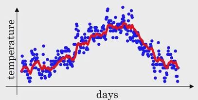
For example we have some measurements x1…x100.
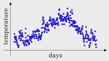
We want to smooth this plot. So we can take:
v0 = 0
v1 = 0.9 * v0 + 0.1 * x1
v2 = 0.9 * v1 + 0.1 * x2
...
v_t = 0.9 * v_(t-1) + 0.1 * x_t
General formula:
v_t = B * v_(t-1) + (1 - B) * x_t
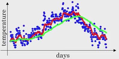
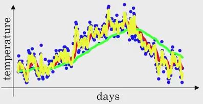
v_t is approximately average over 1/(1-B) measurements.
if B = 0.9 then v_t is an average over ~ 10 measurements.
if B = 0.98 then it averages over ~ 50 measurements.
if B = 0.5 ~ 2 measurements. Each measurement makes a big impact on the result. That's why it is so noisy.
Momentum update
is another approach that almost always enjoys better converge rates on deep networks.
v = mu * v - learning_rate * dx
x += v
where mu is a hyperparameter (typically 0.9).
Initially exp moving average v is 0. And the first update is the same as in vanilla gradient descent.
The parameter vector will build up velocity in any direction that has consistent gradient.
Adagrad
is an adaptive learning rate method.
cache += dx**2
x += - learning_rate * dx / (np.sqrt(cache) + eps)
Variable cache has size equal to the size of the gradient, and keeps track of per-parameter sum of squared gradients. This is then used to normalize the parameter update step, element-wise. The weights that receive high gradients will have their effective learning rate reduced, while weights that receive small or infrequent updates will have their effective learning rate increased. The square root operation turns out to be very important and without it the algorithm performs much worse. eps is used to avoid division by zero (from 1e-4 to 1e-8). A downside of Adagrad is that in case of Deep Learning, the monotonic learning rate usually proves too aggressive and stops learning too early.
RMSprop
Adjusts the Adagrad method in a very simple way in an attempt to reduce its aggressive, monotonically decreasing learning rate. It uses a moving average of squared gradients instead.
cache = decay_rate * cache + (1 - decay_rate) * dx**2
x += - learning_rate * dx / (np.sqrt(cache) + eps)
decay_rate is a hyperparameter and typical values are [0.9, 0.99, 0.999]. Notice that the x+= update is identical to Adagrad, but the cache variable is a “leaky”. Hence, RMSProp still modulates the learning rate of each weight based on the magnitudes of its gradients, which has a beneficial equalizing effect, but unlike Adagrad the updates do not get monotonically smaller.
Adam
Combination of RMSprop with momentum update.
m = beta1*m + (1-beta1)*dx
v = beta2*v + (1-beta2)*(dx**2)
x += - learning_rate * m / (np.sqrt(v) + eps)
The update looks exactly as RMSProp update, except the “smooth” version of the gradient m is used instead of the raw (and perhaps noisy) gradient vector dx. Recommended values in the paper are eps = 1e-8, beta1 = 0.9, beta2 = 0.999. In practice Adam is currently recommended as the default algorithm to use, and often works slightly better than RMSProp. The full Adam update also includes a bias correction mechanism, which compensates for the fact that in the first few time steps the vectors m, v are both initialized and therefore biased at zero, before they fully “warm up”. With the bias correction mechanism, the update looks as follows:
# t is your iteration counter going from 1 to infinity
m = beta1*m + (1-beta1)*dx
mt = m / (1-beta1**t)
v = beta2*v + (1-beta2)*(dx**2)
vt = v / (1-beta2**t)
x += - learning_rate * mt / (np.sqrt(vt) + eps)