Udacity Self-Driving Car Project #2: Traffic sign classification

Overview

The task is to identify which traffic sign is present in an image which has been pre-cropped, presumably by another part of a detection system. The image data is from German Traffic Sign Detection Benchmark (GTSRB) data set.

Dataset Summary & Exploration
First lets load the data set and explore it:

TRAIN_IMAGE_DIR = 'GTSRB\\Final_Training\\Images'

dfs = []
#open csv file
for train_file in glob.glob(os.path.join(TRAIN_IMAGE_DIR, '*/GT-*.csv')):
    folder = train_file.split('\\')[3]
    df = pd.read_csv(train_file, sep=';')
    df['Filename'] = df['Filename'].apply(lambda x: os.path.join(TRAIN_IMAGE_DIR, folder, x))
    dfs.append(df)

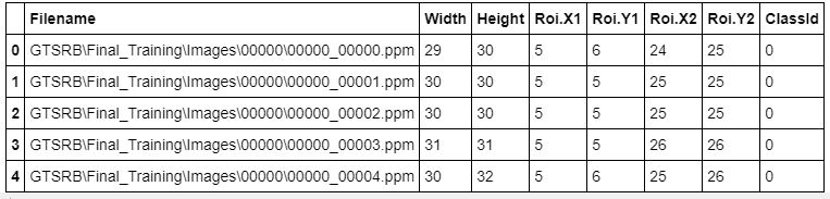
train_df = pd.concat(dfs, ignore_index=True)
train_df.head()

The train data set looks like:

It contains 39209 examples of 43 classes.

Let’s look at a histogramm of class distribution:

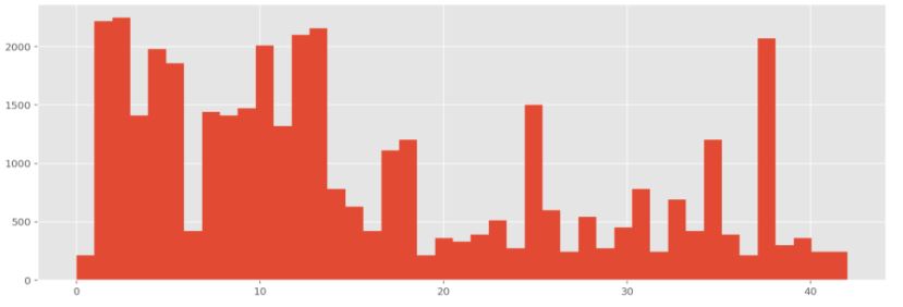
It is clear that the data is unbalanced - some classes have way more examples than other.

Now let’s look at the test data set histogramm (test data set contsists of 12630 examples):

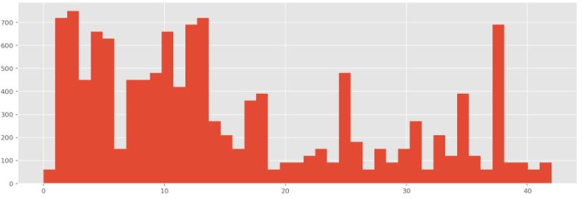
Compare two distributions:

We see that the distributions are almost identical (in percentage of presence) so we may assume that unbalance of the data won’t affect prediction accuracy on the test set.

Let’s see at some examples from the train set. Also print corresponding labels and image size:

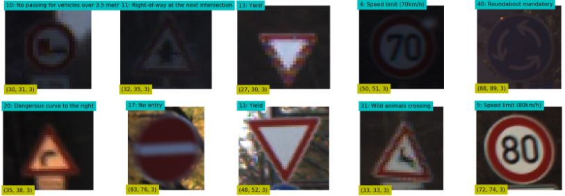
So the images have different resolution. I will resize them to 32x32x1 when doing preprocessing.

Design and Test a Model Architecture

I used a model from a Pierre Sermanet and Yann LeCun paper.

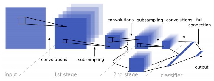
The input is processed in a feedforward manner through two stage of convolutions and subsampling, and finally classified with a linear classifier. The output of the 1st stage is also fed directly to the classifier as higher-resolution features. ReLU activation function was used. I used Dropout technique after first and second convolutions as regularization and Adam optimizer. Also I used exponentially decayed learning rate.

#Stage 1
Input = [N, 32, 32, 1]
Conv1 = [5, 5, 1, 6]
ReLU
MaxPool = [2, 2]
Dropout(keep_prob=0.5)

x1 = [N, 14, 14, 6]

Conv2 = [5, 5, 6, 16]
ReLU
MaxPool = [2, 2]
Dropout(keep_prob=0.5)

x2 = [N, 5, 5, 16]

#Stage 2
Conv3 = [5, 5, 16, 400]
ReLU

x3 = [N, 1, 1, 400]

x4 = concat(flatten(x2), flatten(x3)) = [N, 800]

#Classifier
score = matmul(x4, [800, 43]) = [N, 43]

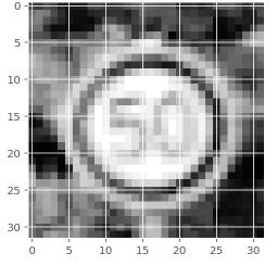
As it was suggested in the paper I converted the images into YUV color space and took only the luma channel (Y) to use it as input for the model. Next the data set of grayscale images is normalized so that the data has mean zero and equal variance. Also I used the histogram normalization technique to correct pixel intensity values (spread pixel intensity distribution).

def preprocess(X, hist=False, normalize=False):
    X = np.array([np.expand_dims(cv2.cvtColor(rgb_img, cv2.COLOR_RGB2YUV)[:,:,0], axis=2) for rgb_img in X])
    if hist == True:
        X = np.array([np.expand_dims(cv2.equalizeHist(np.uint8(img)), axis=2) for img in X])
    if normalize == True:
        X = (X - np.mean(X)) / np.std(X)
    return X

A preproccessed example looks like:

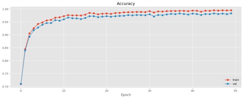
After 50 epoches of training I obtained accuracy on the training data set = 0.995 and on the validation data set = 0.983. The model achieves 0.929 accuracy on the test data set.

Test a Model on New Images

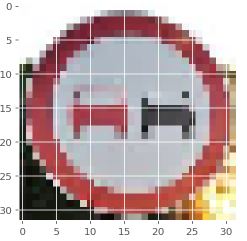
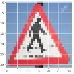
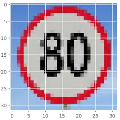
Now I’m going to use the model to predict classes of the images from the Internet. Preprocess them and put labels:

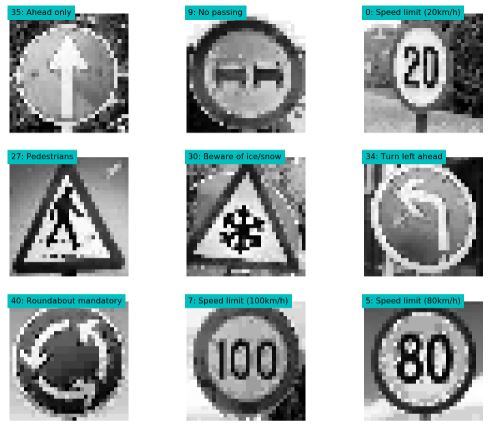
Print 5 best predictions for each image:

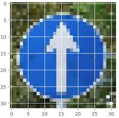
Ahead only  =  99.932 %
Dangerous curve to the left  =  0.029 %
Go straight or right  =  0.016 %
Turn right ahead  =  0.012 %
Right-of-way at the next intersection  =  0.009 %

No passing  =  90.162 %
End of no passing  =  9.531 %
No passing for vehicles over 3.5 metric tons  =  0.280 %
Vehicles over 3.5 metric tons prohibited  =  0.015 %
Ahead only  =  0.003 %

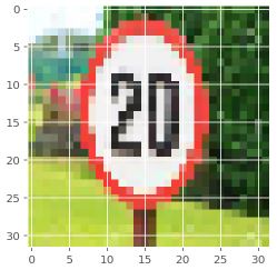
Speed limit (60km/h)  =  49.536 %
Speed limit (20km/h)  =  23.520 %
Roundabout mandatory  =  7.325 %
No passing for vehicles over 3.5 metric tons  =  3.273 %
Priority road  =  2.949 %

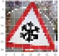
Right-of-way at the next intersection  =  27.180 %
Road narrows on the right  =  24.960 %
Beware of ice/snow  =  18.668 %
Road work  =  10.364 %
Children crossing  =  9.702 %

Children crossing  =  42.562 %
Speed limit (50km/h)  =  15.265 %
Speed limit (60km/h)  =  9.236 %
Road work  =  6.42005354166 %
Speed limit (80km/h)  =  4.657 %

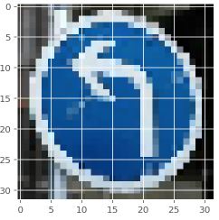
Turn left ahead  =  99.488 %
Keep right  =  0.510 %
Ahead only  =  0.0006 %
Priority road  =  0.0001 %
Road narrows on the right  =  0.0001 %

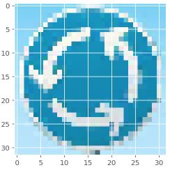
Roundabout mandatory  =  77.899 %
Speed limit (100km/h)  =  19.316 %
Priority road  =  2.406 %
Speed limit (60km/h)  =  0.203 %
Speed limit (80km/h)  =  0.132 %

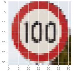
Speed limit (100km/h)  =  55.397 %
Speed limit (120km/h)  =  13.719 %
Vehicles over 3.5 metric tons prohibited  =  11.443 %
Speed limit (20km/h)  =  4.322 %
Right-of-way at the next intersection  =  3.761 %

Speed limit (50km/h)  =  47.604 %
Speed limit (30km/h)  =  27.445 %
Speed limit (60km/h)  =  17.649 %
Speed limit (80km/h)  =  5.681 %
End of speed limit (80km/h)  =  1.328 %

Jupyter Notebook for this project.

The result is 5 correct predictions out of 9 images. Wrong predictions were made for 4 images:

• Pedestrians - the used image is not a German Traffic Sign.
• Beware of ice/snow - 5 best predictions don’t include the right one.
• Speed limit (20km/h) and (60km/h) - the right predictions are in 5 most confident predictions.

Possible improvements

• One possible way to improve accuracy of traffic sign classification is to apply data augmentation techniques so the training dataset contains more diverse examples (I didn’t use this method because training the model on CPU takes too much time).
• Create a trainig data set with the same number of examples for each class (wrong predictions for classes 0 and 30 probably were made because of small amount of examples. As a result the model didn’t learn to generalize well for the unseen images of these classes).