Udacity Self-Driving Car Project #5: Vehicle Detection and Tracking

Overview

The goals of this project is to write a software pipeline to detect vehicles on the road. First, we’ll take a look at classical approach for this problem and after that implement in PyTorch the YOLOv3 - the fastest object detector.

Classical approach

Create robust descriptors for vehicle and non-vehicle objects and train SVM classifier to be able to separate images of those two classes.

Steps to follow:

1.Loading data
Loading data for training SVM classifier is implemented in load_data.py in def load_data(bShuffle=False, cs='YCrCb') function. It loads images both classes (vehicles, non-vehicles) and converts color space to cs. Also data augmentation is performed - each image is horizontally flipped, so the result data set is doubled. Finally the dataset gets shuffled and splitted into train/val sets (90%/10%).
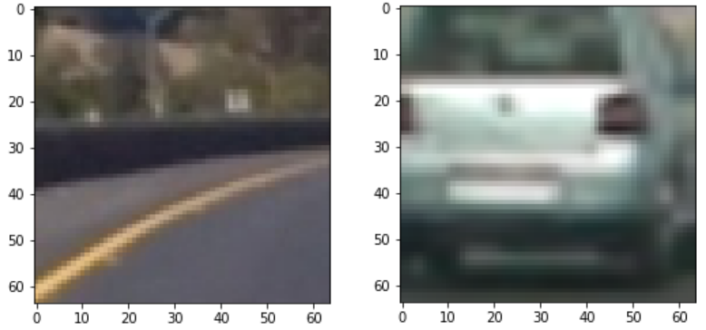
Datasets: Vehicle and Non-vehicle.

Non-vehicle and Vehicle examples

2.Descriptor
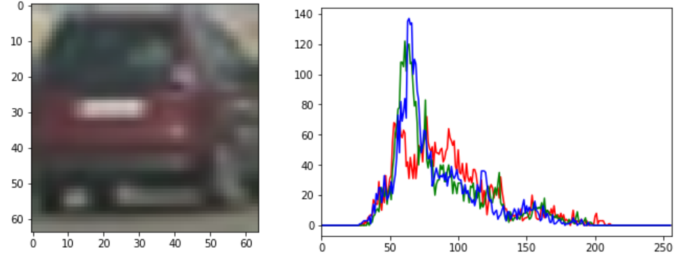
2.1 Histogtram
Calculate histograms for each channel of the crop image (Window) and concatenate them into one vector. Use 256 bins, smaller number of bins affects SVM’s classification.

Histogram for one vehicle example

2.2 Spatial Binning
To add some usefull information to the descriptor resize the crop (Window) to 32x32 pixels and unravel it into a vector.

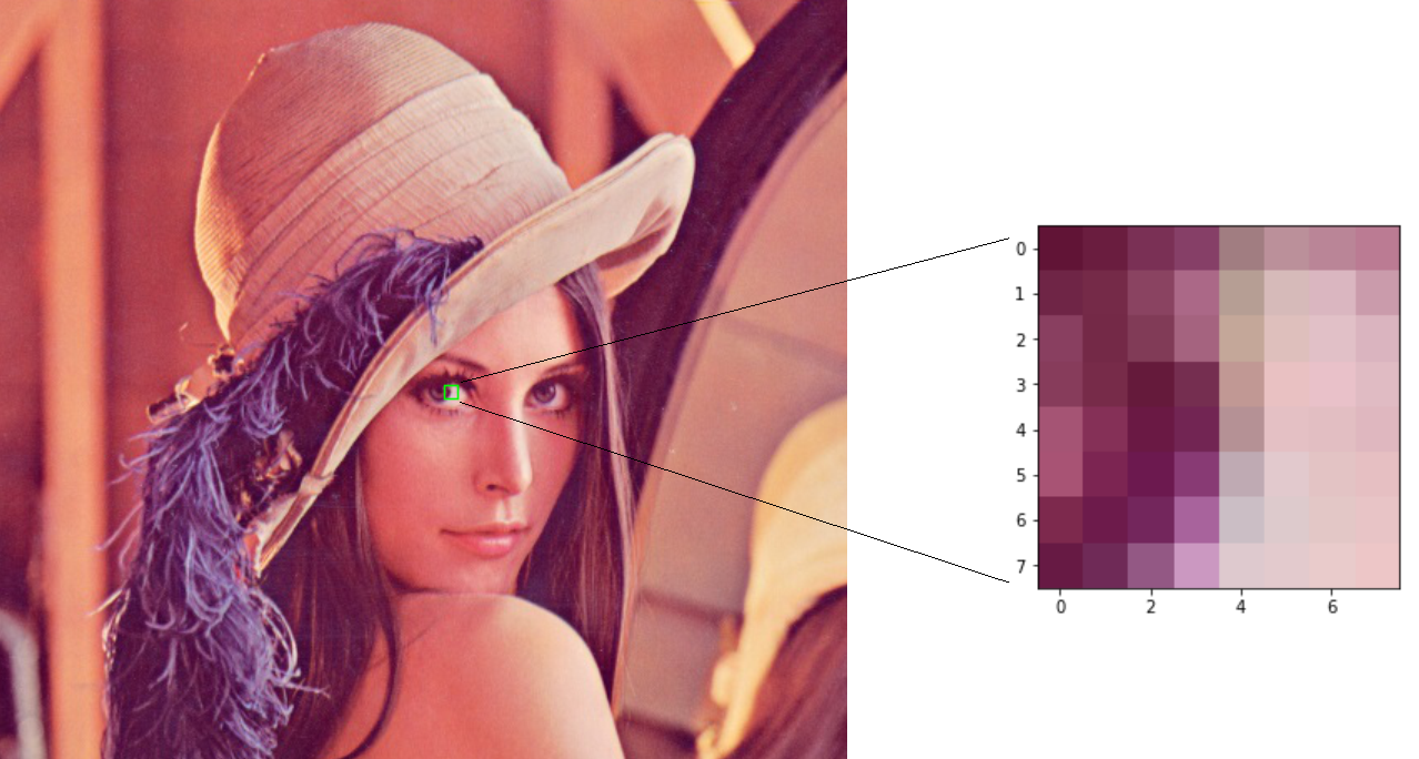
2.3 Historgam of Oriented Gradients (HOG)
First of all gradient of the image is calculated. After calculating the gradient magnitude and orientation, we divide our image into cells and blocks.
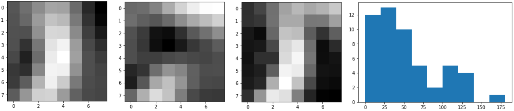
A cel is a rectangular region of pixels that belong to this cell. For example, if we had a 128 x 128 image and defined our pixels_per_cell as 4x4, we would thus have 32 x 32 = 1024 cells.

Pick a cell

Gradient of the cell (Gx, Gy), its magnitute and orientations

Then calculated histograms are normalized. For this step cells are grouped into blocks. For each of the cells in the current block we concatenate their corresponding gradient histograms and perfomr either L1 or L2 normalization of the entire concatenated feature vector. Normalization of HOGs increases performance of the descriptor.

Parameters of the HOG descriptor extractor:
orientations=9 - define the number of bins in the gradient histogram;
pixels_per_cell=(8, 8) - form cells with 8x8 pixels. HOG is calculated for each cell;
cells_per_block=(2, 2) - form blocks of cells, normalize each cell’s HOG wrt the entire block;
blocktransform_sqrt=True - perform normalization;
block_norm="L1" - perform L1 block normalization;
feature_vector=True - return descriptor in vector form (False - roi shape).

Instead of calculating HOG features for each Window in the image do it once for the entire image and then extract features that correspond to the current Sliding Window. This approach improves performance.
HOG explanations 1 and 2.

3.Support Vector Machine (SVM)
Training SVM procedure is implemented in svm.py. First we normalize the image descriptors wiht StandardScaler from sklearn.preprocessing package. Then train a classifier LinearSVC from sklearn.svm. If a validation set is passed to the train_svm function the trained model gets evaluated on val set. Finally the model and the feature scaler are saved as pkl files.

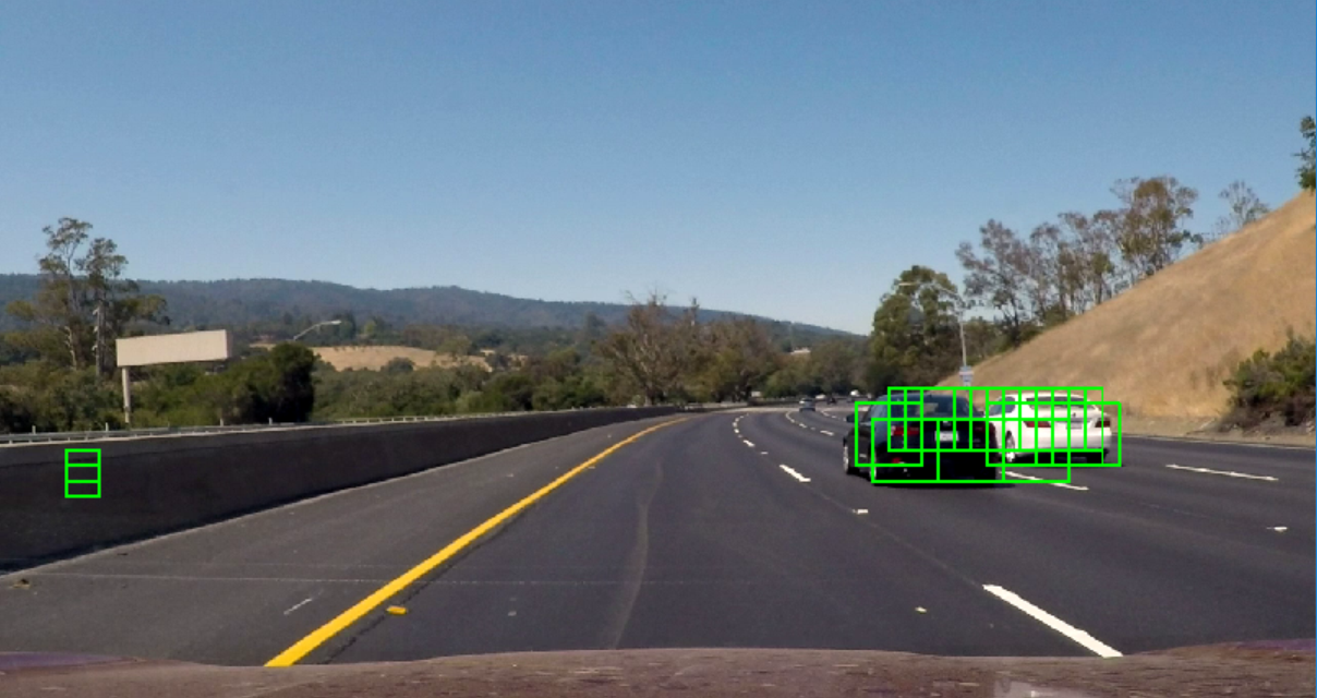
4.Sliding window
Perform Sliding Window technique to look at multiple parts of the image and predict weather there is a car present. Define window parameters (size, stride) in terms of cells. (Implementation details)

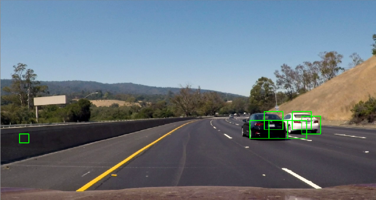
5.Non-Maximum Suppression (NMS)
The algorithm reduces the number of predicted bounding boxes. Pick a box, calculate IoU for this box and the rest of the boxes, discard boxes with IoU > thresh. Repeat. (Great NMS tutorial is here) As a result we have smaller amount of boxes which are stored in a queue to take into acount detections in the previous frames (3 frames).

Detections before NMS

Detections after NMS

6.Heat map
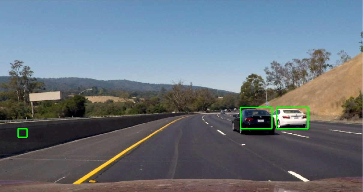
Calculate heat map to combine the detected bounding boxes into several regions which will represent final detections. First we create matrix of zeros with shape as input image. Then we increase the pixel intensity level by 1 at areas corresponding to detected boxes. For example, a pixel at some position of the heat map has value 5. It means that 5 boxes overlap at this position. At the end we binarize the obtained heat map by comparing its values with a threshold. Threshold value allows to choose how many boxes to consider for final detection. With scipy.ndimage.measurements.label function we obtain the segmented heat map (groups of boxes combined into several rectangular areas) and the number of segments. Each segment has different value, we use this knowledge in draw_segment function.

Heat map for detections remained after NMS

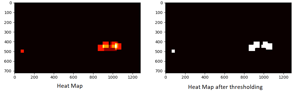
In function draw_segment we interpret the heat map and draw the final detections.

Detections obtained from the heat map

Final video (Classical Approach):

Deep Learning approach

Use object detectors based on deep neural nets. For this step I’ve implemented YOLOv3 detector in PyTorch using this great tutorial.
Code is available here.

Final video (YOLOv3):

Summary

Classical approach allows to detect cars but it is too slow (too far from real time processing). YOLOv3 detector shows more accurate results and much higher processing frame rate (i5-7300 ~ 0.5fps, on Nvidia 920mx ~ 3fps).