Udacity Self-Driving Car Project #6-7: Extended / Unscented Kalman Filters
Both EKF and UKF works well with noisy measurements. However, UKF produces more accurate result wrt minimum of the RMSE. And the results are expected because UKF uses UT instead of linearizing non-linear state/measurement prediction functions (here non-linearity is introduced by radar measurements).
Results EKF (github):
Results UKF (github):
Theory part
Bayes Filter is a recursive algorithm for calculating the belief distribution from measurements and control data (a belief reflects the robot’s internal knowledge about the state of the environment).
Bayes Filter consists of two steps:
- Prediction step. Calculates the beliefe distribution over the current state given previous state and executed control command.
- Update step. Calculated corrected beliefe distribution over the current state \(x_{t}\) by taking into account the sesnor’s data.
Kalman Filter is an implementation of the Bayes Filter. It works under restrictions:
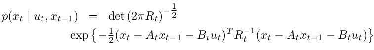
1.The state transition probability \(p(x_{t} | u_{t}, x_{t−1})\) must be a linear function in its arguments with added Gaussian noise

The posterior state probability:
2.The measurement probability \(p(z_{t} | x_{t})\) must also be linear in its arguments, with added Gaussian noise
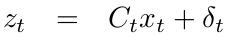
The measurement probability:

3.The initial belief \(bel(x_{0})\) must be normally distributed.

These three assumptions are sufficient to ensure that the posterior \(bel(x_{t})\) is always a Gaussian, for any point in time \(t\) (a linear transformation of Gaussian distribution is still Gaussian).
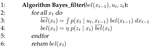
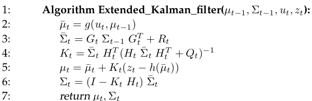
The Kalman filter algorithm:
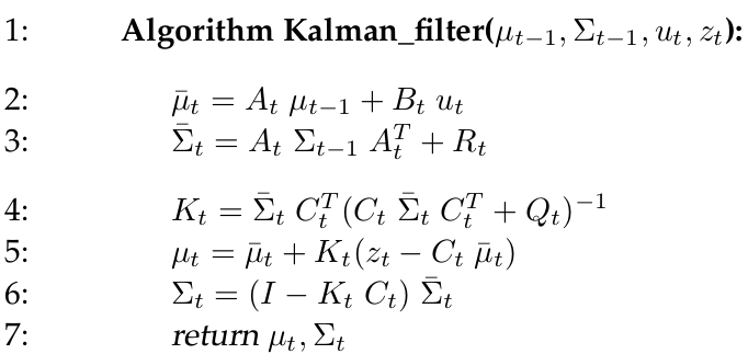
Kalman filters represent the belief \(bel(x_{t})\) at time \(t\) by the mean \(μ_{t}\) and the covariance \(Σ_{t}\). The input of the Kalman filter is the belief at time \(t − 1\), represented by \(μ_{t−1}\) and \(Σ_{t−1}\). To update these parameters, Kalman filters require the control \(u_{t}\) and the measurement \(z_{t}\). The output is the belief at time \(t\), represented by \(μ_{t}\) and \(Σ_{t}\). In lines 2 and 3, the predicted belief \(μ̄\) and \(Σ̄\) is calculated representing the belief \(bel(x_{t})\) one time step later, but before incorporating the measurement \(z_{t}\). This belief is obtained by incorporating the control \(u_{t}\). The mean is updated using the deterministic version of the state transition function, with the mean \(μ_{t−1}\) substituted for the state \(x_{t−1}\). The update of the covariance considers the fact that states depend on previous states through the linear matrix \(A_{t}\). This matrix is multiplied twice into the covariance, since the covariance is a quadratic matrix.
The belief \(bel(x_{t})\) is subsequently transformed into the desired belief \(bel(x_{t})\) in lines 4 through 6, by incorporating the measurement \(z_{t}\). The variable \(K_{t}\), computed in line 4 is called Kalman gain. It specifies the degree to which the measurement is incorporated into the new state estimate. Line 5 manipulates the mean,
by adjusting it in proportion to the Kalman gain \(K_{t}\) and the deviation of the actual measurement, \(z_{t}\), and the measurement predicted according to the measurement probability. The key concept here is the innovation, which
is the difference between the actual measurement \(z_{t}\) and the expected measurement \(C_{t} μ̄_{t}\) in line 5. Finally, the new covariance of the posterior belief is calculated in line 6, adjusting for the information gain resulting from the measurement.
The Kalman filter is computationally quite efficient. For today’s best algorithms, the complexity of matrix inversion is approximately \(O(d^{2.4})\) for a matrix of size \(d × d\). Each iteration of the Kalman filter algorithm, as stated here, is lower bounded by (approximately) \(O(k^{2.4})\), where \(k\) is the dimension of the measurement vector \(z_{t}\). This (approximate) cubic complexity stems from the matrix inversion in line 4.
In many applications—such as the robot mapping applications the measurement space is much lower dimensional than the
state space, and the update is dominated by the \(O(n^{2})\) operations.
The extended Kalman filter
The assumptions that observations are linear functions of the state and that the next state is a linear function of the previous state are crucial for the correctness of the Kalman filter. The observation that any linear transformation of a Gaussian random variable results in another Gaussian random variable played an important role in the derivation of the Kalman filter algorithm. The efficiency of the Kalman filter is then due to the fact that the parameters
of the resulting Gaussian can be computed in closed form.
Unfortunately, state transitions and measurements are rarely linear in practice. For example, a robot that moves with constant translational and rotational velocity typically moves on a circular trajectory, which cannot be described by linear state transitions.
The extended Kalman filter, or EKF, relaxes one of these assumptions: the linearity assumption. Here the assumption is that the state transition probability and the measurement probabilities are governed by nonlinear functions \(g\) and \(h\), respectively:
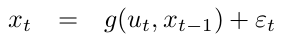
This model strictly generalizes the linear Gaussian model underlying Kalman filters. The function \(g\) replaces the matrices \(A_{t}\) and \(B_{t}\) and \(h\) replaces the matrix \(C_{t}\). Unfortunately, with arbitrary functions \(g\) and \(h\), the belief is no longer a Gaussian. In fact, performing the belief update exactly is usually impossible for nonlinear functions \(g\) and \(h\), and the Bayes filter does not possess a closed-form solution.
Linearization Via Taylor Expansion
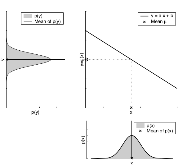
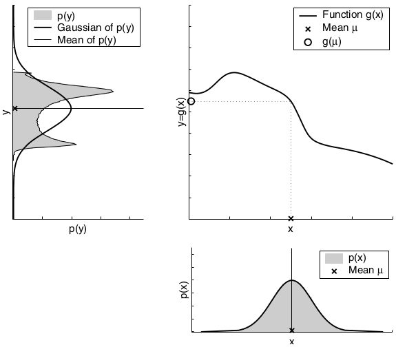
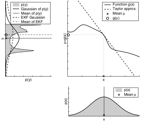
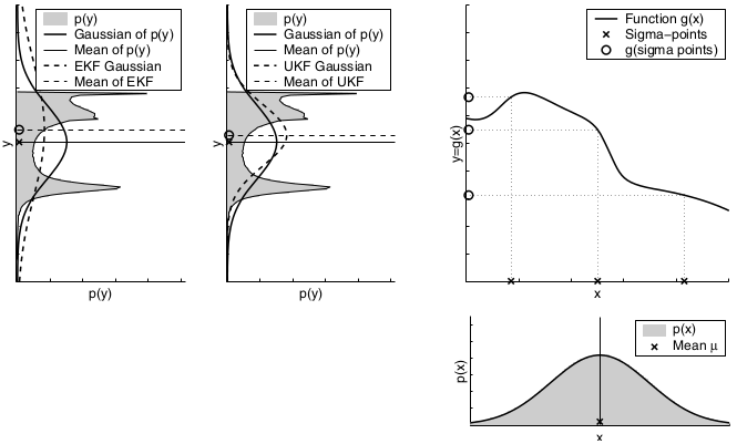
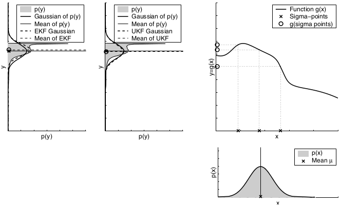
The key idea underlying the EKF approximation is called linearization. Linearization approximates the nonlinear function \(g\) by a linear function that is tangent to \(g\) at the mean of the Gaussian. Projecting the Gaussian through this linear approximation results in a Gaussian density. The solid line in the upper left graph represents the mean and covariance of the Monte-Carlo approximation. The mismatch between these two Gaussians indicates the error caused by the linear approximation of \(g\).
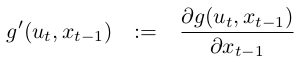
The key advantage of the linearization, however, lies in its efficiency. The Monte-Carlo estimate of the Gaussian was achieved by passing 500,000 points through \(g\) followed by the computation of their mean and covariance. The linearization applied by the EKF, on the other hand, only requires determination of the linear approximation followed by the closed-form computation of the resulting Gaussian. In fact, once \(g\) is linearized, the mechanics of the EKF’s belief propagation are equivalent to those of the Kalman filter. This technique also is applied to the multiplication of Gaussians when a measurement function \(h\) is involved. Again, the EKF approximates \(h\) by a linear function tangent to \(h\), thereby retaining the Gaussian nature of the posterior belief. There exist many techniques for linearizing nonlinear functions. EKFs utilize a method called (first order) Taylor expansion. Taylor expansion constructs a linear approximation to a function \(g\) from \(g’\) value and slope. The slope is given by the partial derivative:
\(g\) is approximated by its value at \(μ_{t−1}\) (and at \(u_{t}\), and the linear extrapolation is achieved by a term proportional to the gradient of \(g\) at \(μ_{t−1}\) and \(u_{t}\):
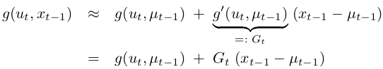
The state transition probability is approximated as follows:
Notice that \(G_{t}\) is a matrix of size n × n, with n denoting the dimension of the state. This matrix is often called the Jacobian. The value of the Jacobian depends on \(u_{t}\) and \(μ_{t−1}\), hence it differs for different points in time. EKFs implement the exact same linearization for the measurement function \(h\). Here the Taylor expansion is developed around \(μ̄_{t}\), the state deemed most likely by the robot at the time it linearizes \(h\):
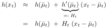
The measurement probability:
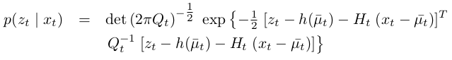
That is, the linear predictions in Kalman filters are replaced by their nonlinear generalizations in EKFs. Moreover, EKFs use Jacobians \(G_{t}\) and \(H_{t}\) instead of the corresponding linear system matrices \(A_{t}\) , \(B_{t}\) , and \(C_{t}\) in Kalman filters. The Jacobian \(G_{t}\) corresponds to the matrices \(A_{t}\) and \(B_{t}\), and the Jacobian \(H_{t}\) corresponds to \(C_{t}\).
An important limitation of the EKF arises from the fact that it approximates state transitions and measurements using linear Taylor expansions. In most robotics problems, state transitions and measurements are nonlinear. The goodness of the linear approximation applied by the EKF depends on two main factors:
1.The degree of uncertainty
2.The degree of local nonlinearity of the functions that are being approximated.
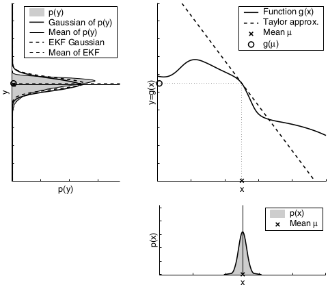
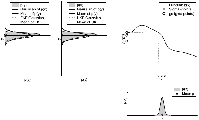
A comparison to the Gaussians resulting from the Monte-Carlo approximations illustrates the fact that higher uncertainty typically results in less accurate estimates of the mean and covariance of the resulting random variable.
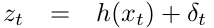
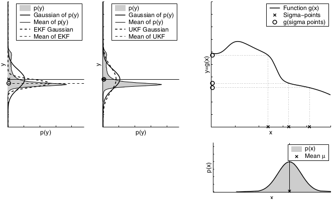
The second factor for the quality of the linear Gaussian approximation is the local nonlinearity of the function \(g\).
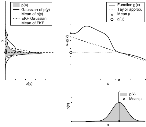
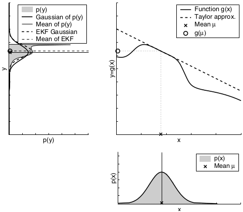
The mismatch between the accurate Monte-Carlo estimate of the Gaussian (solid line, upper left) and the Gaussian resulting from linear approximation (dashed line) shows that higher nonlinearities result in larger approximation errors. The EKF Gaussian clearly underestimates the spread of the resulting density.
To summarize, if the nonlinear functions are approximately linear at the mean of the estimate, then the EKF approximation may generally be a good one, and EKFs may approximate the posterior belief with sufficient accuracy. Furthermore, the less certain the robot, the wider its Gaussian belief, and the more it is affected by nonlinearities in the state transition and measurement functions. In practice, when applying EKFs it is therefore important to keep the uncertainty of the state estimate small.
The Unscented Kalman Filter
Another linearization method is applied by the unscented Kalman filter, or UKF, which performs a stochastic linearization through the use of a weighted statistical linear regression process.
Linearization Via the Unscented Transform
The UKF deterministically extracts so-called sigma points from the Gaussian and passes these through \(g\).
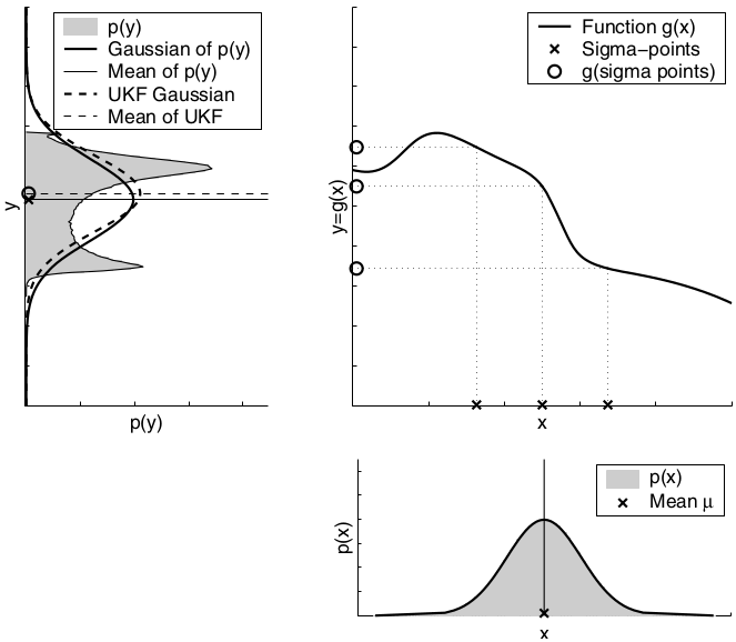
In the general case, these sigma points are located at the mean and symmetrically along the main axes of the covariance (two per dimension). For an n-dimensional Gaussian with mean \(μ\) and covariance \(Σ\), the resulting 2n + 1 sigma points \(X^{[i]}\) are chosen according to the following rule:
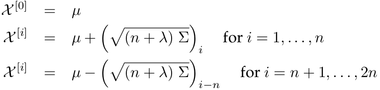
Here \(λ = α^2*(n+κ)−n\), with \(α\) and \(κ\) being scaling parameters that determine how far the sigma points are spread from the mean. Each sigma point \(X^{[i]}\) has two weights associated with it. One weight, \(w_{m}^{[i]}\), is used when computing the mean, the other weight, \(w_{c}^{[i]}\), is used when recovering the covariance of the Gaussian.
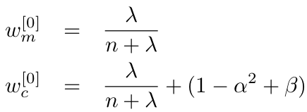
The parameter \(β\) can be chosen to encode additional (higher order) know ledge about the distribution underlying the Gaussian representation. If the distribution is an exact Gaussian, then \(β = 2\) is the optimal choice. The sigma points are then passed through the function \(g\), thereby probing how \(g\) changes the shape of the Gaussian.
The parameters \((μ’ Σ’)\) of the resulting Gaussian are extracted from the mapped sigma points \(Y^{[i]}\) according to
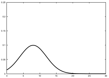
The dependency of the unscented transform on the uncertainty of the original Gaussian:
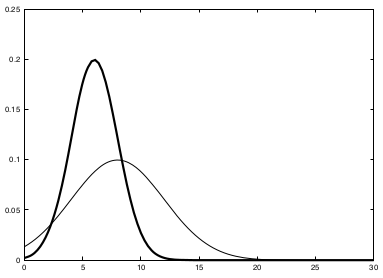
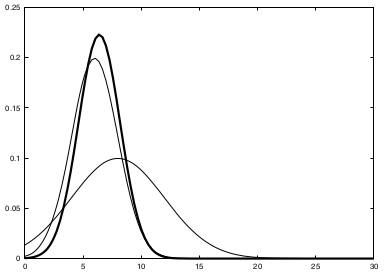
Dependency of the local nonlinearity of the function \(g\). As can be seen, the unscented transform is more accurate than the first order Taylor series expansion applied by the EKF. In fact, it can be shown that the unscented transform is accurate in the first two terms of the Taylor expansion, while the EKF captures only the first order term. (It should be noted, however, that both the EKF and the UKF can be modified to capture higher order terms.)
The UKF Algorithm
The UKF algorithm utilizes the unscented transform.
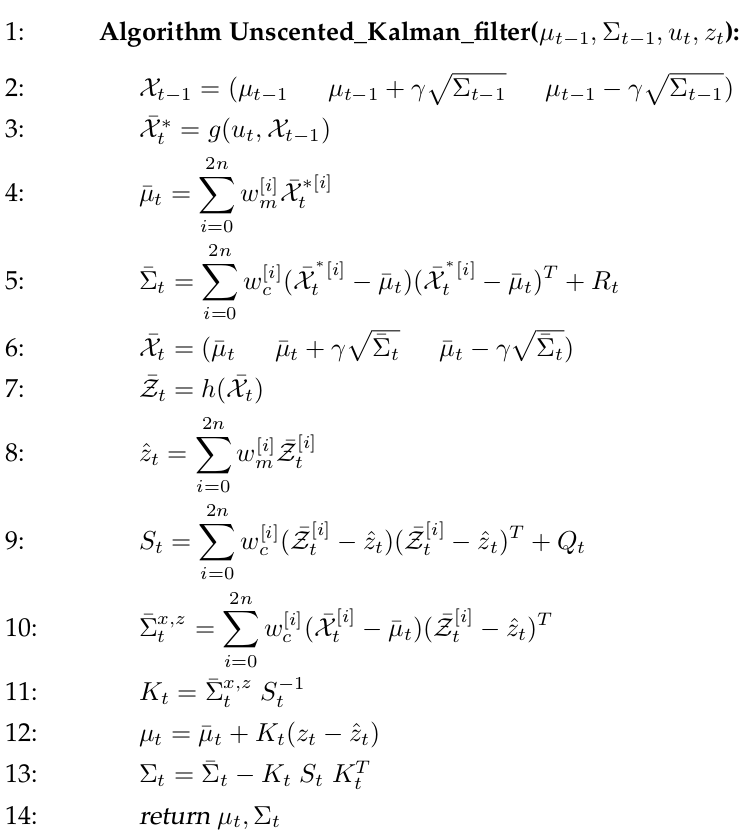
The input and output are identical to the EKF algorithm. Line 2 determines the sigma points of the previous belief, with \(γ\) short for \(√(n + λ)\). These points are propagated through the noise-free state prediction in line 3. The predicted mean and variance are then computed from the resulting sigma points (lines 4 and 5). \(R_{t}\) in line 5 is added to the sigma point covariance in order to model the additional prediction noise uncertainty (compare line 3 of the EKF algorithm in Table 3.3). The prediction noise \(R_{t}\) is assumed to be additive. A new set of sigma points is extracted from the predicted Gaussian in line 6. This sigma point set \(X̄_{t}\) now captures the overall uncertainty after the prediction step. In line 7, a predicted observation is computed for each sigma point. The resulting observation sigma points \(Z̄_{t}\) are used to compute the predicted observation \(ẑ_{t}\) and its uncertainty, \(S_{t}\). The matrix \(Q_{t}\) is the covariance matrix of the additive measurement noise. Note that \(S_{t}\) represents the same uncertainty as \(H_{t}Σ̄_{t}H_{t}^T + Q_{t}\) in line 4 of the EKF algorithm. Line 10 determines the cross-covariance between state and observation, which is then used in line 11 to compute the Kalman gain \(K_{t}\). The cross-covariance \(Σ̄_t^{x,z}\) corresponds to the term \(Σ̄_{t} H_{t}^T\) in line 4 of the EKF algorithm. With this in mind it is straightforward to show that the estimation update performed in lines 12 and 13 is of equivalent form to the update performed by the EKF algorithm.
The asymptotic complexity of the UKF algorithm is the same as for the EKF. In practice, the EKF is often slightly faster than the UKF. The UKF is still highly efficient, even with this slowdown by a constant factor. Furthermore, the UKF inherits the benefits of the unscented transform for linearization. For purely linear systems, it can be shown that the estimates generated by the UKF are identical to those generated by the Kalman filter. For nonlinear systems the UKF produces equal or better results than the EKF, where the improvement over the EKF depends on the nonlinearities and spread of the prior state uncertainty. In many practical applications, the difference between EKF and UKF is negligible.
Another advantage of the UKF is the fact that it does not require the computation of Jacobians, which are difficult to determine in some domains. The UKF is thus often referred to as a derivative-free filter.
Materials:
- Online lections: SLAM course by Cyrill Stachniss
- Probabilistic Robotics by Sebastian Thrun, Wolfram Burgard and Dieter Fox